ROC curve and AUR in the simplest way
In this blog, we will learn about validation matrices. One such way is by observing the ROC curve of the model.
by the end of this blog, you will learn,
- What are true positive, true negative, false positive and false negative values?
- What is confusion matrix, what does it signify?
- What is the ROC curve?
- Why do we need ROC curve?
- Which threshold value is best for our model?
- What is Area Under the Curve (AUC), what does it represent?
- How to compare two or models with the help of ROC curves?
Let’s take a simple example,
Suppose we have created a model which predicts whether a patient has cancer or not. Our data has 1 for positive cancer and 0 for negative cancer (benign) as an output. Here, we are not focusing on our model but its outcome. Our model is a binary classifier which is also a probabilistic model.
If you are a doctor, you want your model to be 100% accurate because cancer is a serious disease, and you don’t want to give your patients false treatment.
So it is very important to choose good validation metrics.
Accuracy
The most obvious choice of this is Accuracy metrics. The accuracy is the no. of correctly classified samples divided by the total no. of samples. This will give us how accurate our model is.
Suppose there are 1000 samples in the test set from which 70% of the samples are of positive cancer (1) and 30% are negative samples. If we want to apply a naive model which predicts 1 for every patient, we will have an accuracy of 70%.
Do you see the problem here? Even if we apply a model which is random, we get very decent accuracy. (what if we had 90% samples with the positive case?)
How would you solve this problem then?
Before we go there, let’s go step by step, and understand the basics first.
True Positive, True Negative, False Positive and False Negative
There are four values that we need to know.
- True Positive: The patient is cancer positive, our model predicted he/she is positive
- True Negative: The patient is cancer negative(benign), our model predicted he/she is negative
- False Positive: The patient is cancer negative but our model predicted he/she is positive
- False Negative: The patient is cancer positive but our model predicted he/she is negative
We do not want our model to give more false negatives, because, as you may understand, this will cause serious trouble. We can handle a few false positives for now. If the use-case is cost-sensitive then this should be below as well.
Now we know, accuracy alone is not a good measure. Accuracy can be tricky on skewed data.
Before we go further, we need some data to play with, it will help us understand this all better,
y_true = [ 0, 0, 0, 0, 1, 0, 1,
           0, 0, 1, 0, 1, 0, 0, 1]
y_pred = [ 0.1, 0.3, 0.2, 0.6, 0.8, 0.05, 0.9,
           0.5, 0.3, 0.66, 0.3, 0.2, 0.85, 0.15, 0.99]
Our model gives the probability of being positive(cancer). It is a non-linear model which means, it does not tell us the actual output. We need to decide the threshold for that.
Threshold Value
A threshold value is a value above which (or below which) we decide if the certain probability is valid is positive.
If we pick a threshold of 0.5, i.e., if our model predicts more than 0.5, it will predict it to be positive, and below 0.5, it would be negative.
Now our models output will look something like this,
threshold = 0.5
y_output = [1 if x >= threshold else 0 for x in y_pred]
print(y_output)
[0, 0, 0, 1, 1, 0, 1, 1, 0, 1, 0, 0, 1, 0, 1]
We can find the accuracy of the model in the following way using scikit-learn (You can write your function for finding accuracy)
>>from sklearn import metrics
>>accuracy = metrics.accuracy_score(y_true, y_output)
>>print(accuracy)
0.7333333333333333
Not bad, but we already know that accuracy is not the correct validation metrics.
So, let’s find out those four values first, using following code,
def true_positive(y_true, y_pred):
    tp = 0
    for yt, yp in zip(y_true, y_pred):
        if yt == 1 and yp == 1:
            tp += 1
    return tp

def true_negative(y_true, y_pred):
    tn = 0
    for yt, yp in zip(y_true, y_pred):
        if yt == 0 and yp == 0:
            tn += 1
    return tn

def false_positive(y_true, y_pred):
    fp = 0
    for yt, yp in zip(y_true, y_pred):
        if yt == 0 and yp == 1:
            fp += 1
    return fp

def false_negative(y_true, y_pred):
    fn = 0
    for yt, yp in zip(y_true, y_pred):
        if yt == 1 and yp == 0:
              fn += 1
    return fn
Let’s calculate these values,
tp = true_positive(y_true, y_output)
tn = true_negative(y_true, y_output)
fp = false_positive(y_true, y_output)
fn = false_negative(y_true, y_output)

print("True Positive", tp)
print("True Negative", tn)
print("False Positive", fp)
print("False Negative", fn)

### OUTPUT ###
True Positive 4
True Negative 7
False Positive 3
False Negative 1
To find out what is happening, we should make a confusion matrix. It is nothing but putting those four values together.
Confusion Matrix
| Cancer Negative | Cancer Positive | |
| Cancer Negative | True Negative | False Positive |
| Cancer Positive | False Negative | True Positive |
We can put those values as they are, but we can use scikit-learn to calculate confusion matrix as well
metrics.confusion_(y_true, y_output)

### OUTPUT ###
array([[7, 3],
       [1, 4]])
But, what is the confusion matrix? when do we need it? what does it represent?
What does the confusion matrix represent?
We need this confusion matrix to tell us two different things (for now). Firstly, we need it to tell us how good our model is in predicting the positive outcome correctly. This value tells us the true positive rate (TPR) or sensitivity of the model.
By TPR we mean, how good is our model in predicting true cancer patients out of total correctly predicted cancer patients (out of both positive and negative).
So, formula for the FPR or Sensitivity is,
tpr = true_positive/ (true_positive + false_negative)Secondly, we want to know how good is our model in predicting negative class. We need to find; how good is our model in predicting no-cancer out of the total no. of no-cancer predictions. This value tells us the false positive rate (FPR).
We can go a little further, we can find out the total no of false negative samples, 1-FPR (see the equation below) and this tells us the specificity of the model. It is the true negative rate(TNR). You can use TNR instead of FPR for ROC curves. But for now, let’s just go with FPR and TPR
fpr = false_positive/ (true_negative + false_positive)ROC curve
Well, now that we know about all the basics. So, let’s come to our main topic, finally, the ROC curve, which is a short form for Receiver Operating Characteristics. This curve tells us which threshold to use for our prediction.
Now, remember we used 0.5 as our threshold. We considered, if our model’s output is above 0.5 then it’s positive cancer and below 0.5 is negative cancer. We chose this on our own, randomly. Our probabilistic model will always give us the probability values for both positive and negative. The last task from our end would be to decide what our threshold should be.
Here come those TPR and FPR values. Again, remember that TPR calculates how good is our model in predicting positive samples and FPR calculates how wrong is our model in predicting positive samples. So, for good predictions, we want our model to have low FPR and high TPR, at a certain threshold.
Let’s go on and find our TPR and FPR values for 0.5 threshold as before.
tpr = tp/ (tp + fn)
fpr = fp/ (tn + fp)

### OUTPUT ###
TPR 0.8
FPR 0.3
We can change our threshold value to 0.1 and then see the results.
True Positive 5
True Negative 1
False Positive 9
False Negative 0

TPR 1.0
FPR 0.9
Multiple Thresholds
Let’s check it for every multiple thresholds,
y_true = [ 0, 0, 0, 0, 1, 0, 1,
           0, 0, 1, 0, 1, 0, 0, 1]
y_pred = [ 0.1, 0.3, 0.2, 0.6, 0.8, 0.05, 0.9,
           0.5, 0.3, 0.66, 0.3, 0.2, 0.85, 0.15, 0.99]

# checking multiple thresholds
thresholds = [0.0, 0.1, 0.2, 0.3, 0.4, 0.5, 0.6, 0.7, 0.8, 0.9, 1.0]

tprs = []
fprs = []
for threshold in thresholds:
    y_output = [1 if x>=threshold else 0 for x in y_pred]
    tp = true_positive(y_true, y_output)
    tn = true_negative(y_true, y_output)
    fp = false_positive(y_true, y_output)
    fn = false_negative(y_true, y_output)
    tpr = tp/ (tp + fn)
    fpr = fp/ (tn + fp)
    tprs.append(tpr)
    fprs.append(fpr)

df = pd.DataFrame({'Threshold': thresholds, 'TPR': tprs, 'FPR': fprs)
print(df)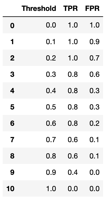
As we increase the threshold, we make our model harder to predict 1. And that is why we see the True Positive Rate decreasing in the above table. As the true positive rate decreases, the false positive rate also decreases(mostly). Because, if it is hard enough to predict actual true value it will be even harder to predict false positive value.
Finding best threshold
So, what should be our threshold? We should keep our threshold in such a way that our true positive rate is as high and our false positive rate as low as possible.
To visualise this, we can plot a graph like below,
import matplotlib.pyplot as plt

plt.figure(figsize = (8, 8))
plt.fill_between(fprs, tprs, alpha = 0.4)
plt.plot(fprs, tprs, lw = 7)
plt.xlim(0, 1.0)
plt.ylim(0, 1.0)
plt.xlabel('FPR', fontsize = 15)
plt.ylabel('TPR', fontsize = 15)
plt.show()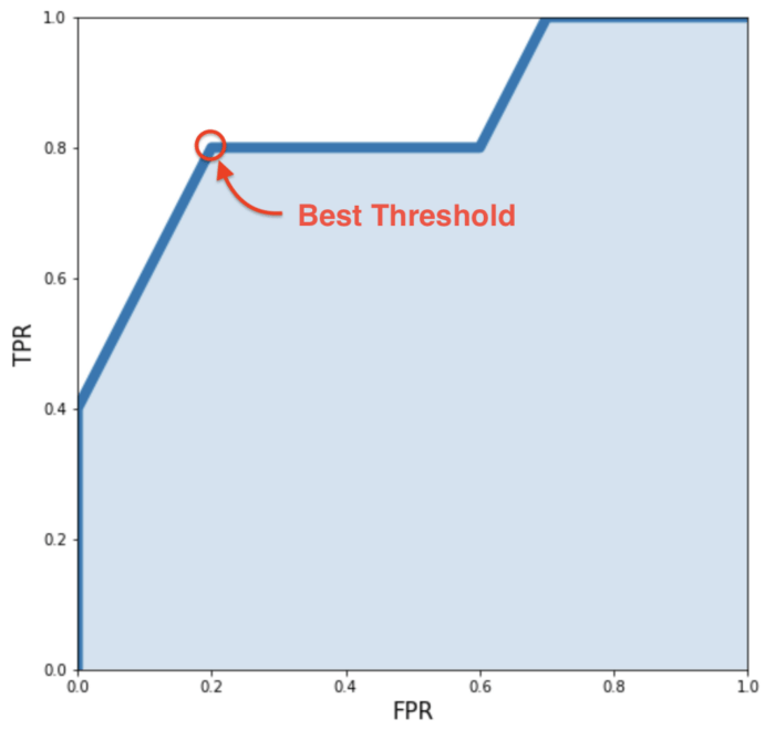
As we want low FPR and high TPR, we should be looking for a point closest to the top-left corner. And we can see (0.2, 0.8) i.e 0.6 threshold gives the best results for our model.
Good enough!
But did we do this just for a good threshold? No, there’s one more concept in this story.
What is AUR? (Area Under the Curve)
As the name suggests, this is the area under the ROC curve. Now, what’s the significance of this?
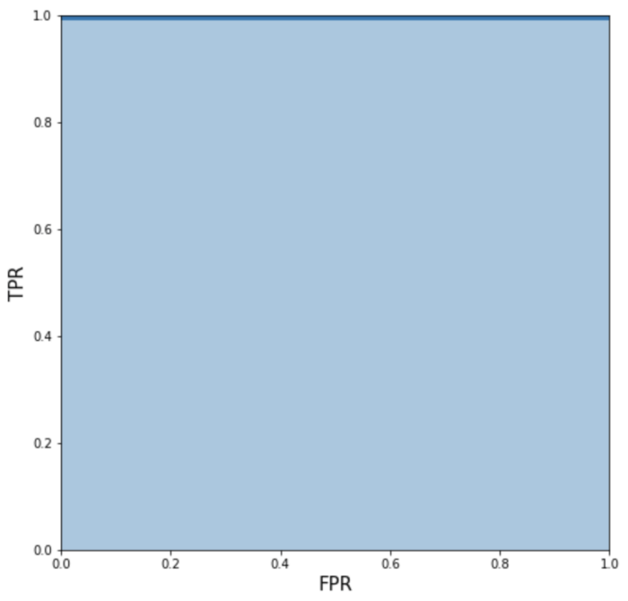
A good model will always give us high TPR (always 1) at any threshold. And for the FPR values, it will always give us zero, except for the threshold 0 where it would be 1 (as at 0 thresholds our model will consider all values to be true and hence false positive rate would be 1). If we plot this graph we will get AOR 1.
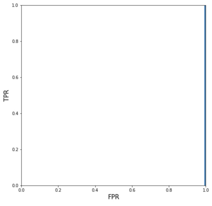
On the other hand, if our model is extremely useless, we should have AOR 1 because in that case, we will have FPR 1 and TPR always 0 except for 0 thresholds (same as above). If we plot it, we get AOR 0.
AOR of 0.5 is just a random guess. Any model with a random guess can produce an AOR of about 0.5.
For any reason, our model has AOR less than 0.5, which means, we must have flipped the results and after switching then again it will show more than 0.5.
But wait there’s one more thing we can use from AOR.
Comparing two (or more) models with ROC
If we have multiple models, let’s say we have a KNN model and another is Random Forest model to predict cancer patients like above. We can compare these two models based on AOR and select the best fit.
y_true = [ 0, 0, 0, 0, 1, 0, 1,
           0, 0, 1, 0, 1, 0, 0, 1]
y_pred = [ 0.1, 0.3, 0.2, 0.6, 0.8, 0.05, 0.9,
           0.5, 0.3, 0.66, 0.3, 0.2, 0.85, 0.15, 0.99]

# let's take another model
y_pred1 = [ 0.6, 0.4, 0.1, 0.3, 0.9, 0.15, 0.95,
           0.7, 0.4, 0.5, 0.6, 0.4, 0.95, 0.10, 0.80]
and if we plot ROC curve for these together, we get the following.
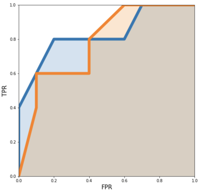
Now let’s find out the AOR,
model1_AOR = metrics.roc_auc_score(y_true, y_pred)
model2_AOR = metrics.roc_auc_score(y_true, y_pred1)

print("AOR model1:", model1_AOR)
print("AOR model2:", model2_AOR)

### OUTPUT ###
AOR model1: 0.8300000000000001
AOR model2: 0.77
A model that has AOR closer to 1 would be closer to an ideal model, that is, a model that has high AOR would be better than the model which has low AOR.
In this case, model1 has more AOR than model2. And hence, this is how we can compare two (or more) models.
There’s more, to learn about precision and recall, read this blog!
Hopefully, this helped you. Consider subscribing to the newsletter for latest updates! Hit me anytime on Twitter, LinkedIn!
Leave a Reply